We continue with the post dedicated to giving a small overview of automatic control systems in a processor like Arduino. In this post we will see the PID controller, one of the most widespread controllers due to its simplicity and its ability to achieve good behavior in a wide variety of situations.
In the first post we saw some generalities and definitions about control theory. In the second, we saw one of the simplest controls, the on/off control with hysteresis, as well as its limitations.
Of course, we insist that we will not go into the details of the PID, as it is a very extensive (and interesting) topic. If you are interested, you can consult the abundant documentation available.
Here we will try to give an intuitive view of the controller and the motivation that explains its behavior. Without using equations or mathematics. In fact, that’s one of the great things about PID: you don’t need to know in detail how it works to make it work.
What is the PID controller?
The PID controller is one of the most used in industry for controlling feedback systems. Some of its strengths are its simplicity and its ability to provide good behavior in a wide variety of situations without needing to know the plant to be controlled in detail.
The PID controller has been known for a long time. Its first uses date back to 1911, and its first theoretical analysis was in 1922 by Nicolas Minorsky. In those times, PID control was exclusively analog. However, it is easy to implement a digital PID in programming and the calculations it requires are simple and efficient. Furthermore, it is “relatively easy” to extrapolate the theory of analog PIDs to their digital equivalent.
Despite its popularity, we must say that currently the PID is not the best controller available. But in most cases it is more than enough. On the other hand, many of the more “modern” controllers are nothing more than improved versions of a PID, such as the various families based on PID with adaptive parameters.
How does PID work?
The PID algorithm (proportional, integral, derivative) is formed by the sum of three components, Proportional, Integral, and Derivative. Mathematically, a PID controller has the following formulation.
Wait a minute, wait a minute. We said no equations! Well yes, but we can’t do a post about PID without seeing at least its formulation. I promise there won’t be any more, okay?
Each component of the PID is “independent” of the others, in the sense that each one calculates an output of what “for it” you should do to get the appropriate response.
The three components are added together to give the controller’s output. Each one fulfills a certain function and improves a certain part of the response. And when the three components work together, in the right proportion, they achieve great behavior.
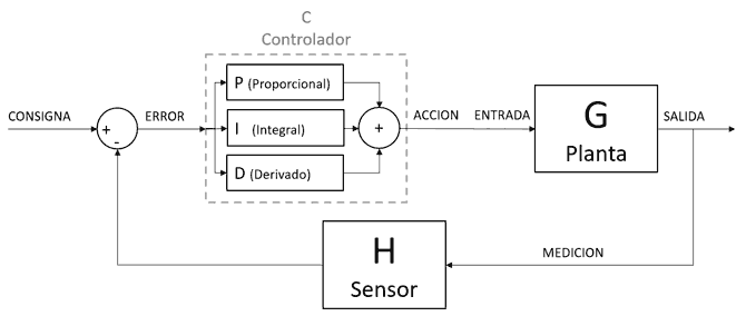
Each component has a parameter Kp, Ki and Kd, respectively. These parameters indicate the weighting (or “the strength”) it has in the final result. Whether the PID’s response is good, broken things, death, destruction, and firing, lies in the correct tuning of these three parameters.
And here comes the “funny” part of PID. In the three parameters, if you set a value too low, the effect of the component on the output won’t be noticeable. And if you set it too high… well, that’s it, death, destruction, broken things, etc.
Furthermore, in the overall response of the controller, the three components work together and influence each other, so it’s not enough to adjust each parameter independently. There is a certain “zone” within the three parameters where the behavior is more or less good.
Logically, it is clear that the difficulty (which isn’t that great either) of a PID is adjusting the parameters K, Ki and Kd so that the behavior is good. And that’s what we’ll dedicate the next post to.
Explaining the PID
To explain the PID controller, we are going to continue with our example. Let’s remember that in this case you are the controller and you are sitting in a room. On the wall you have two displays, one blue and one red. You also have a lever.
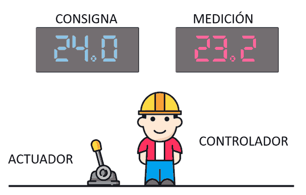
All you know is that the lever controls the power of a building’s climate control system. The red number is the building’s actual temperature, and the blue one is the one we want it to be. Your mission, logically, is for the building’s actual temperature to equal the setpoint.
Beyond that, you know nothing. You don’t know what the building is like, what your climate control system is like, if all the windows have been opened, if 100 people enter the building, if it’s dawn, if it’s winter. You don’t even know if moving the lever causes a small effect, or if you’re going to scorch someone.
On the positive side, we have a continuous (or semi-continuous) input and output, which is a requirement for PID control. As we saw in the previous one, if the sensor or actuator were of the on/off type, we would have to go for an on/off controller or a hysteresis controller.
As we said, the PID controller is based on three components, PID. Its “strength” lies in the role each of these components plays in the response. As a summary, so you have it in your head.
- The proportional component reacts to the present
- The integral component reacts to the past, and provides “memory” to the controller.
- The derivative component reacts to the future, and provides “prediction” to the controller
Next, we are going to go into depth on each of the components, seeing their motivation, operation, and behavior.
PID Simulation
So you can check the behavior of the PID components, we have this simulation where you can adjust the values of Kp, Ki and Kd to visualize the influence of each parameter on the output, and on the action requested by the controller.
Move the Kp, Ki and Kd Sliders to see the changes in the controller’s response.
PID Components
For this we will use our simple example that you have woken up in the middle of a control room, knowing nothing else. Unless we say otherwise, the setpoint (blue screen) is always at 24ºC.
Motivation
The motivation for the proportional component is probably the most intuitive to explain. If you enter the room and see 12ºC, it seems logical that you have to push the lever more than if it says 23ºC. Right?
Well, that’s the motivation of the proportional component, it makes sense that you apply more action the further you are from the desired value, and vice versa.
Formulation
The proportional component is calculated simply as a factor K multiplied by the error (difference between setpoint and actual value).
Behavior
The proportional factor has a great influence on the response speed of the system. If we have a small K, the system will take a long time to reach the setpoint, because we are giving “little power” to the actuator. If we increase it, we can reduce the response time.
But if we increase K too much we can overshoot the setpoint, oscillate, or even oscillate and send everything to hell. Let’s see how that happens.
If you have a K that is too large, you are going to push the lever too much. So when you see 18ºC, you push the lever and the next value is 25. You’ve overshot. You lower the lever, 21, now you’ve overshot downwards. You raise the lever, 23. Good, you’ve got it.
But if you have an even larger K, it could happen that when you see 18º you push the lever A LOT, and the next thing you see could be 32ºC. Wow, I’ve overshot a lot, LOWER THE LEVER! 14º WOW RAISE RAISE! 45º… 8º… 56º… You’ve just made your system oscillate and become unstable (death, destruction…).
Another characteristic is that, in general, the proportional component does not completely eliminate the error in the long term. In our example, suppose that at 22ºC and a certain lever position, the energy we supply to the building is exactly what the building needs to maintain the temperature. We would have managed to stabilize the temperature, but since the lever position is given by the error (which has stabilized) we will never be able to raise the 2ºC we are missing.
Motivation
The function of the integral component is perhaps the most difficult to explain within the PID. Imagine you are in the room, and we have the 22ºC we had before. The proportional tells you to put the lever in a position and you put it there. A minute passes, another passes, another passes… and it’s still at 22ºC, 2ºC below what we want.
The integral component is the one that says… hey guys, maybe we should raise the lever a bit, no? Because we’ve been at 22ºC for a good while without moving the lever, and it doesn’t look like it’s going to go away. Well, that voice with so much sense, which reacts to the memory of past error, is the integral component.
Formulation
The integral component applies an action that is proportional to the integral of the error over time. Equivalently, it responds proportionally to the sum of all previous errors.
Graphically it corresponds to the area enclosed under the error curve, which is also the same as the area between the output and the setpoint. In the discrete domain, the integral is replaced by a discrete method for its calculation, such as calculation using rectangles or trapezoids.
Behavior
The integral component allows the controller to completely eliminate the error in the long term. However, if Ki is very small, the system will take a long time to eliminate the error.
On the other hand, keep in mind that the integral term only responds to the area between the output and the setpoint. A consequence of this is that if we have accumulated (for example) an error by being below the setpoint, the only way the integral term has to compensate for it is to be above for a while.
And indeed, the integral component has a tendency to overshoot and oscillate, even more than the proportional term.
Motivation
The derivative component is also easy to explain. Let’s say you are calmly with the temperature at the setpoint of 24ºC. Perfect! The temperature drops to 23ºC, then to 22ºC, and you raise the lever a little. All good, very calm.
Now imagine that, when you were at 24ºC, the temperature suddenly drops to 18ºC. Wow, that’s a big drop. You raise the lever. It reads 12ºC … I don’t know if they opened a window or what’s happening, but this is dropping very fast! Next value 2ºC PUSH PUSH PUSH, it’s getting out of hand by the second!
That is the function of the derivative component, to react to variations in error (due to setpoint change or variable change). Because it’s not the same to be at 12ºC and rising slowly, than if the temperature is plummeting at full speed. That is, the derivative term responds to the rate of change of the error.
Formulation
The derivative component is calculated proportionally to the derivative of the error with respect to time at the present moment. Equivalently, it responds proportionally to the difference between the current error and the error at the previous instant.
In the discrete domain, the derivative is replaced by the difference between the current error and the previous error, divided by the sampling time (or this division is omitted entirely and included in the Kd coefficient, if the sampling time is constant).
Behavior
The derivative component improves the overall response of many systems for moderate Kd values. However, if we overdo Kd we will see a lack of “smoothness” in the response, and other “weird” behaviors.
Furthermore, the derivative component responds very poorly to measurement noise. Noise, a high-frequency variation, implies very rapid variations, even if they are of small amplitude. These variations are amplified by the derivative component.
And finally, the derivative component is sometimes a bit “brutal” because it demands very large actions. Imagine, for example, an instantaneous change in the setpoint. The derivative component would demand an infinite action that the actuator could not satisfy. Since the actuator could not provide the action requested by the controller, we would have deviations from what was calculated, or we could even damage the actuator.
Conclusion
We have seen the PID controller, one of the most used and versatile PID controllers that can control a wide variety of systems with good results, without needing to characterize the plant.
The behavior of the PID is based on the sum of its three components, which are controlled through the constants Kp, Ki and Kd. The three constants have to be calibrated for the plant to be controlled, and on this adjustment depends whether the system’s response is good, bad, or very very bad.
The process of adjusting the constants is called “tuning” a PID controller, and in the next post in the series we will see different strategies for tuning the PID. See you soon!