Explanation of Nyquist Sampling Theorem without Equations

New entry in this series I love about explaining mathematics and engineering concepts without equations. This time we get to see the Nyquist-Shannon Sampling Theorem.

For those who don’t know it, the sampling theorem was formulated by Nyquist in 1928, and proven by Shannon in 1949, and is one of the cornerstones of digital signal processing.

The most well-known formulation of the theorem is that to be able to reconstruct a sampled signal, the sampling frequency must be greater than twice the bandwidth.

And now normally a mathematical spiel would follow to prove this. Which is precisely NOT the goal of this post, but quite the opposite.

Don’t get me wrong, I love equations. But if explaining something requires two pages of math, maybe your teacher didn’t fully understand it (and you risk forgetting it in a ‘snap’).

So, what’s all this mystique and endless articles about the “saaaampling theoreeeem” about? But, before we get to that, we need to start by remembering what a sampled signal is.

Sampled Signals

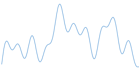
Let’s assume a “real” signal from the physical world, such as an audio signal or an electromagnetic one. In general, these “real” signals are variations in the measurement of a magnitude. With few (and contrived) exceptions, physical signals are always analog.

In this context, momentarily away from the blackboard and the math book, by “real” and analog we mean signals that are not continuous, not periodic, with infinite detail and even their fair share of noise. A real signal party, in short.

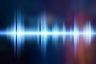
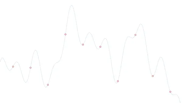
For example, the following is an audio signal captured with a microphone.

If I want to digitally store this “real” analog signal, it doesn’t fit. I would need infinite memory to store its infinite level of detail. So I have to simplify it somehow. And simplifying almost always means losing information.

The simplest and most intuitive way to digitize our “real” signal is to sample it, that is, take measurements at regular intervals and store them. This list of numbers is our digital signal.

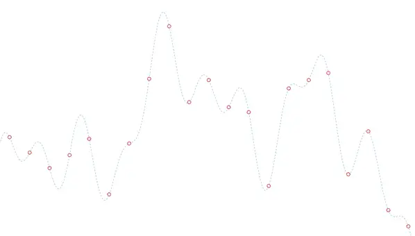
Then, if I have to reconstruct the analog signal from the data, I have various ways, like “playing connect the dots”, or more or less sophisticated interpolations, depending on how much I want to strain my brain and how much computing power I have.

An obvious characteristic of the sampling process is that the closer the points are, i.e., the higher my sampling frequency, the more details of the signal I will capture.

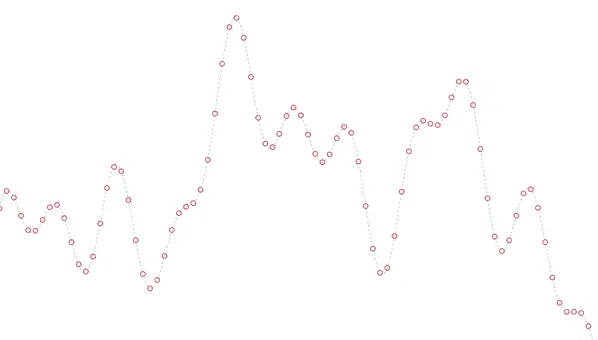
And conversely, if I space them further and further apart, I’ll end up with a potato of a digital signal, because if my sampling frequency is very small compared to the signal’s frequency, I lose a lot of information. Between two points there can be a peak, a smooth curve, 20 oscillations… a camel, an elephant, anything (which, on the other hand, may or may not interest me).

Well, this same thing worried Nyquist, Shannon (and others) 100 years ago, and that’s what the sampling theorem is about, how the spacing between points affects the quality of the sampled signal.

Signal Spectrum

Our “real” signal is continuous, infinitely detailed, and also made up. I’ll draw one, and you’ll draw a different one. So we won’t be able to draw many conclusions this way.

To draw relevant theoretical conclusions it is convenient to move to the frequency domain, that is, to look at the signal in an alternative representation as a summation of sinusoidal signals.

To go from the time domain to the frequency domain we use the Fourier integral Transform. Specifically, we will use one of its versions such as the DFT (Discrete Fourier Transform) and the FFT algorithm (Fast Fourier Transform). But, for our explanation, it’s the same.

This transform allows us to treat (or see, or conceive) our signal in a different way, but without changing it (that’s why it’s a transform, not a Fourier change). Simply, instead of treating it as a function of the signal’s magnitude at each instant of time, now we treat it as a function that encodes the amplitude of its frequency components.

By moving our signal to the frequency domain, we obtain this function which we will call the spectrum of the function. If our “real” function was continuous, non-periodic, blah blah blah…, its spectrum will also be continuous, non-periodic, with noise, blah blah blah.

So what’s the point then? Why have we done all this? Because now, if we can know what happens to a sinusoidal signal of a certain frequency when we sample it, we can deduce what will happen to the “real” signal (or at least part of it) when we sample it.

Well, let’s go, let’s take our signal from the previous point and do a Fourier transform on it and we see… that I’ve tricked you. Actually, I generated it with the sum of four sine signals, with made-up frequencies and amplitudes.

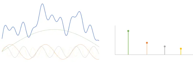
Well, what did you expect, I already told you you can’t store a “real” signal. And it has served us to visualize its frequency components. But keep in mind that in a “real” signal its spectrum would be continuous, and instead of four points, we would have a continuous curve.

Representation Using Phasors

The previous section served to conclude that we are going to work with the signal in its frequency domain. This way, we only need to work with sinusoidal signals to extract valid consequences about how sampling affects “real” signals.

Time for another tool, which is the treatment of sinusoidal signals using their phasor representation. And what the heck is this now? A ball that spins, but the names don’t help make this seem simple.

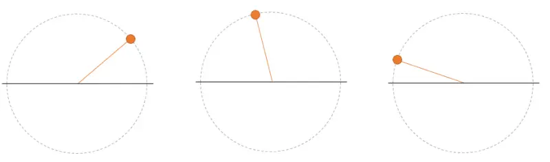
You may remember from high school that a sinusoid (sine, cosine) is actually the projection of a point that is spinning around a center. In fact, every time a phenomenon that follows a sinusoidal pattern appears in nature, it’s because it’s related to something that spins, and you’re looking at it wrong. But that’s another debate.

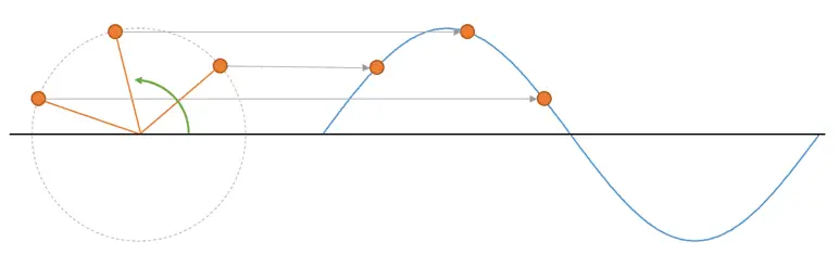
This is a phasor representation and it greatly simplifies working with sinusoids. The radius of the phasor’s spin relative to the center is the amplitude of the wave, and the frequency of the sinusoid is the frequency at which the phasor spins, which is equivalent to its spin speed.

With this in mind, we have enough tools to understand the sampling theorem.

The Sampling Problem

Recentering the topic, the sampling problem roughly boils down to knowing if we can reconstruct a signal from the sampled “points”, or at least what consequences the process has on the sampled signal compared to the original.

By moving to the frequency domain, the problem has become, given that series of points, can you tell me the sinusoidal signals that best fit that series of points? Darn… it’s even worse than before! How am I supposed to know that?!

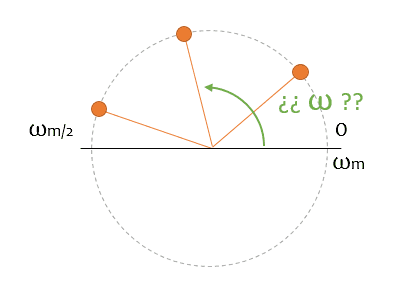
No, it’s not that hard anymore. If we work in phasors, the question ends up being, can you tell me for each of the following balls, its frequency and its spin radius? And that’s very easy, because each ball spins at a different speed.

Since I can easily discriminate each “ball” (frequency component) simply because they go at different speeds, I can focus the analysis on just one frequency, and the rest of the analysis will be similar for all components.

So now I only care about, for example, the red ball. After sampling, I have “static images” (samples) of the ball in its motion. We just have to calculate its angular velocity, to determine the frequency component.

And that’s very easy! Or is it? Hint, if it were that easy we wouldn’t be here. This is about to get interesting.

Fundamental Harmonics

First difficulty, but not too problematic. You see the following ball (let’s call it a phasor from now on, okay?) spinning, and calculating the spin speed is trivial. Right?

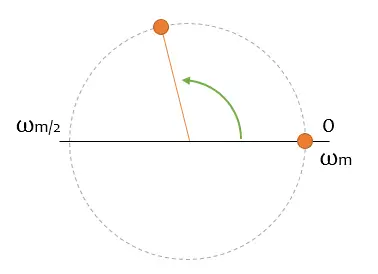
Well, yes and no. Because you only have two static images, and you don’t know if between them, the phasor has made 10, 20, or three million turns (remember? a camel, an elephant…). In all cases, the ball would be at the same point in the second photo.

That is a first problem of sampling, that you have an uncertainty about which harmonic you are representing. In general, it’s not a big problem because you know you are sampling at a frequency Wm, so any higher frequency is “reasonably” assumed that you are going to lose it.

But, it’s important for you to keep in mind for the following sections that the speed (frequency) that I’m going to assume you want when we do the reconstruction is the lowest possible one.

Explanation of the Sampling Theorem

We finally get to the “core” of the post. What happens when we increase the frequency of the component in relation to the sampling frequency? (either because we increase the component’s frequency, or because we reduce the sampling frequency).

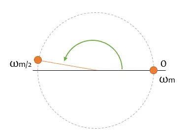
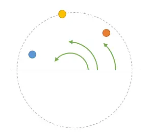
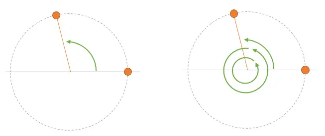
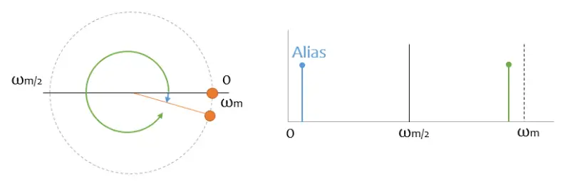
Well, so far no problems. Let’s increase the phasor’s spin speed a little more, until it crosses the abscissa axis. What will happen then?

Wow! You expected the green arrow to get a little bigger, but instead a blue one has appeared. Oh, hadn’t I said that phasors can spin in both directions? Well yes, they spin in both directions.

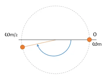
And remember, from the previous section, I told you I was going to tell you the lowest speed of all possible ones. As soon as you cross the abscissa axis, I think it’s spinning in the opposite direction.

We finally arrive at our demonstration without equations. If you want me to reconstruct a frequency, I need to have at least two samples in the same half of the circle. That is, its frequency must be lower than half of my sampling frequency.

Equivalently, it means I cannot reconstruct frequency components higher than half the sampling frequency, which is exactly what we wanted to prove.

Aliasing

Did you think this ended here? There’s still a little bit left. Now it’s time to talk about another consequence, less known and much less understood, of the sampling theorem, the terrible and horrible Aliasing.

I’m sorry to tell you I’ve been lying to you for half the post. Remember I told you I was only going to give you the lowest frequency component? Well, that’s a lie, I’m always going to give you both directions of spin.

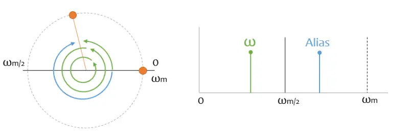
Remember the first example of the phasor, where it was very easy to determine the frequency. Let’s plot it together with its spectrum.

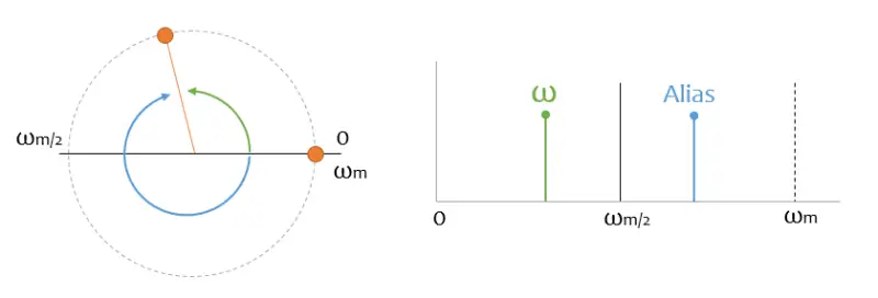
Actually, I’m not only going to have a green peak, but I’m also going to have a blue one, which corresponds to the frequency spinning in the other direction. This “mirror” signal is called an “alias”, and it is what gives rise to the phenomenon of Aliasing.

This peak doesn’t seem very problematic, because it’s above half the sampling frequency. And, since we are smart guys, and thanks to the genius of Nyquist and Shannon, I know that everything above is “garbage” and I won’t even look at it when reconstructing the signal.

If only it were that easy. But look what happens with a noise “somewhat above” half the sampling frequency, which appears to me as a high frequency in my sampled digital signal! And I can’t distinguish it from the “real” data!

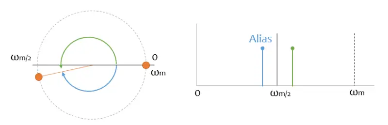
It’s even worse if it gets close to the sampling signal, because it appears to me as low-frequency components in my digital signal. And it’s worse because, normally, in the low frequencies I have a lot of the “meat” of my signal.

But not only that, also all the harmonics of frequencies above half the sampling frequency will generate Aliasing for me.

In general, when I do a sampling process of a signal, I am sampling the “mirror” of its entire spectrum and all its harmonics. And all that signal is being “eaten up” and I have no way to distinguish it from the “real” data.

That’s why, always always always, before sampling a signal it is necessary to filter for bands above half the sampling frequency, to prevent all that information from sneaking into the recorded spectrum.

Conclusion

A bit long? I hope it wasn’t too tedious, and that you’ve seen a different way to understand the sampling theorem, without the need for equations (very beautiful ones, by the way).

The sampling theorem is applicable in multiple fields, typically in telecommunications and audio, but also in many other less obvious ones like image processing (yes, 2D and 3D FFTs exist), oscilloscopes, measurement instruments, and in any application that involves digital manipulation of signals.

So let’s thank the geniuses Nyquist, Shannon and other contributors to the theory of digital information processing for their work and see you in the next post!