Measure inclination with IMU, Arduino and complementary filter

In previous posts we have seen the operation of accelerometers and gyroscopes as sensors that can be used to determine the orientation of a device.

We also saw the advantages and limitations of each of the devices, and we anticipated that they combine very well because the characteristics of their measurement complement each other.

In this last post of the series, we will see the IMUs, devices that combine the advantages of both sensors to obtain better functionalities than we could obtain using an accelerometer or gyroscope independently.

Currently, their low cost has made them frequent components in a large number of everyday devices. There are many manufacturers of IMUs, such as Panasonic, Robert Bosch GmbH, InvenSense, Seiko Epson, Sensonor, STMicroelectronics, Freescale Semiconductor, and AnalogDevices.

We will use them frequently in our electronics and Arduino projects, for example, to determine the forward direction of a vehicle, the orientation of an actuator, the inclination of a platform, or even as a way to interact with a computer with a glove or a 3D mouse.

What is an IMU?

An inertial measurement unit (IMU) is the generic name for a device that is capable of measuring the velocity, orientation, and acceleration of a system.

When talking about IMUs, it is common to refer to the number of degrees of freedom (DOF) available. The degrees of freedom of a sensor represent the number of independent magnitudes it is capable of measuring.

Thus, a 3-axis orthogonal accelerometer is a 3 DOF sensor. Likewise, a gyroscope that measures angles in 3 orthogonal axes is a 3DOF sensor.

The IMUs that we will most frequently find are:

• 6 DOF IMU, combining a 3-axis accelerometer and a 3-axis gyroscope.
• 9 DOF IMU, adding a 3-axis magnetic compass.
• 10 DOF IMU, which adds a barometer for estimating the sensor’s height.

As we can see, most IMUs start with a combination of accelerometer and gyroscope, with this being the most common IMU. The reason is that both devices combine very well and compensate for each other’s limitations.

• Accelerometers do not have medium or long-term drift because they measure the absolute angle formed by the sensor with the vertical direction, marked by gravity. However, they are influenced by the movements of the sensor and noise, so they are not reliable in the short term.
• Gyroscopes work very well for short or sudden movements, but when using gyroscopes of vibration that actually measure the angular velocity, and obtain the angle by integration over time, they accumulate errors and noise in the measurement, so they have medium or long-term drift.

Therefore, combining the measurements of both devices allows IMUs to obtain more precise orientation measurements than an accelerometer and a gyroscope separately. We will see this below, but first, we will reflect on what orientation is.

Obtaining orientation with an IMU

To determine the distribution of an object with respect to a base in a three-dimensional space we must establish its position and orientation. Three parameters are required to determine the relative position and three more to determine its orientation.

In everyday life, we are used to dealing with the position of an object, and we know that there is more than one way to express its relative position mathematically. For example, we can express its coordinates relative to another base, using Cartesian coordinates (X, Y, Z), cylindrical or spherical coordinates.

However, we are not so used to working with the parameterization of orientation, as mathematically it is somewhat more complex. Like position, there is more than one way to express the relative orientation of two systems, such as Euler angles, rotation matrices, or quaternions.

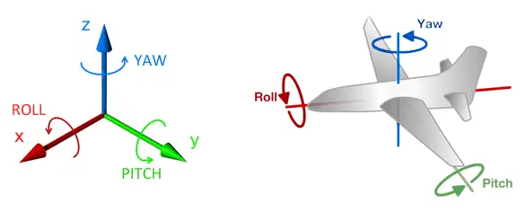
Surely the most widespread and intuitive are the navigation angles, or Tait-Bryan angles, in which the orientation is represented as three orthogonal rotations around the X (roll), Y (pitch), and Z (yaw) axes.

The Tait-Bryan angles are a variation of the Euler angles, introduced by the mathematician Leonhard Euler during his study of the mechanics of rigid bodies.

Tait-Bryan angles are intuitive and simple. They also have the advantage of being commutative, i.e., the final orientation obtained is independent of the order in which we apply the rotation (something that normally does not occur in the representation of rotations).

However, they suffer from a major disadvantage called gimbal lock that all Euler angle systems suffer from. When the Y-axis rotates +-90º, the X and Z axes coincide, so the system degenerates to 2DOF, which leads to a nondifferentiable singular point that can cause stability problems in the calculations.

Gimbal lock is such an important disadvantage that the usual way to represent rotation is by using quaternions. Quaternions are an extension of complex numbers introduced by Hamilton in 1843, which use three imaginary units i, j, and k such that,

It is known that complex numbers can be used to represent vectors in the plane. Similarly, a quaternion allows expressing a vector in three-dimensional space.

To express the rotation of a point, an angle α, around an arbitrary vector of coordinates Ex, Ey, Ez, the resulting quaternion adopts the following expression

Compared to Euler angles, quaternions are simpler to compose and avoid the problem of gimbal lock. Compared to rotation matrices, they are more efficient and more numerically stable.

For this reason, quaternions are one of the most common ways to express orientation in computer graphics and they will be the preferred form to use when working with orientations in IMUs and Arduino projects.

Signal filtering in an IMU

In order to take advantage of the short-term benefits of the gyroscope and the medium and long-term benefits of the accelerometer it is necessary to combine and filter the raw signal.

There are several possible filters, with the most famous being the Kalman filter, developed in 1960 by Rudolf E. Kalman. It is considered one of the great discoveries of the 20th century due to its implications in the sensor filtering process (not only IMUs) and is one of the architects of the space race.

In broad strokes, the Kalman filter makes an estimation of the future value of the measurement, and then compares the real value through a statistical analysis to compensate for the error in future measurements.

However, the general version of the Kalman filter involves complex calculations (see Wikipedia) that imply an excessive implementation and calculation time for Arduino.

For this reason, it is common to use a simpler filter called the complementary filter. In reality, the complementary filter can be considered a simplification of the Kalman filter that completely dispenses with the statistical analysis.

There are several formulations for a complementary filter. In its simplest expression, the complementary filter can be expressed.

Where A and B are two constants that, initially, can be taken as 0.98 and 0.02 respectively. We can calibrate the filter simply by varying the values of A and B as long as we comply with the condition that they sum to 1 between them.

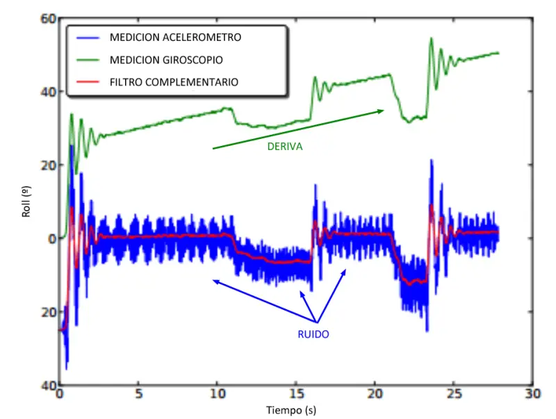
The complementary filter behaves as a high-pass filter for the gyroscope measurement and a low-pass filter for the accelerometer signal. That is, the gyroscope signal sends a short-term signal, and the accelerometer sends a medium and long-term signal, which is exactly what we want to compensate for their advantages and disadvantages.

In most domestic applications, the complementary filter is sufficient and provides values very similar to the Kalman filter, as long as the values of A and B are properly calibrated.

There are more sophisticated versions of the complementary filter, as well as simplified one-dimensional versions of the Kalman filter that can be implemented in Arduino. We will see this in an upcoming advanced post.

In the meantime, we will use IMUs such as the MPU6050 and the filters in our electronics and Arduino projects.

Download the code

All the code from this post is available for download on Github.